G-Art is a transdisciplinary research group with one side towards computer science and the other aiming at arts. As such, some of our works start with strong scientific goals while others are just driven by the pleasure of playing with code letting us see where it goes. Code is here considered as an artistic medium such as painting or ceramics.
It was the case with FlowAutomaton, an experiment we implemented with hoca, our
higher-order cellular automata Python library.
This class of automata produces altered versions of images as the one
we displayed at the
Paradoxes
exhibition (2020), called
A dialog between Leonardo da Vinci and Norbert Wiener.
We did many other experiments with these automata like the video below.
The secret expectation of such experiments is to produce artworks with a pleasing or interesting aesthetic, and it was the case (at least in our opinion). But along the way, there are sometimes interesting questions from a scientific point of view. This is, moreover, the justification of our transdisciplinary approach.
Observing a data-driven behaviour
In the above video, one can remark some thin straight lines and some curvy ones. There are also tiny dots and little circles. All of these features are produced by a population of the same automata class instances running the same very simple code. The Python code excerpt below shows the code shared by all the instances. It has been simplified for readability and for keeping us focused on the important part.
    def __init__(self, automata_population):
        # keep a shortcut to the fields, it improves readability
        self.source_field = self.automata_population.field_dict['source']
        self.destination_field = self.automata_population.field_dict['result']

        # set an initial random position for the automaton
        self.x = random.randint(0, self.source_field.width - 1)
        self.y = random.randint(0, self.source_field.height - 1)

        # select a random direction for (the next move of) the automaton
        self._direction = random.randint(0, 7)

    def run(self):
        # get the grayscale value
        gray = self.source_field[self.x, self.y]

        # update the result field with the grayscale value
        self.destination_field[self.x, self.y] = gray

        # update the automaton memory by computing and storing
        # the new direction of the automaton
        # grayscale value is in [0, 1] and we want an int as the direction in [0, 8]
        # (direction 8 is the same as direction 0)
        self._direction = self._direction + int((gray * 8) - 4)

        # update automaton position
        dx, dy = AutomataUtilities.get_dx_dy(self._direction)
        self.x += dx
        self.y += dy
Feel free to read the hoca library documentation for a more in depth
explanation of a code like this.
So, the question is: How all these graphic behaviours can emerge from
such a simple implementation?
Even if we were surprised by the results, there is no magic here.
As all the instances share the same code, the answer to this question
is obviously in the data processed.
More precisely, the observed behaviours must come from the relationship
between the grayscale value of the pixel under an automaton and the direction
it takes from this value as expressed by the code:
self._direction = self._direction + int((gray * 8) - 4)
Conducting some experiments
We performed experiments with some images specially built: An all black image and an all white one, two gradient images one going horizontally from black to white and one going vertically.
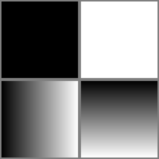
After running some FlowAutomaton instances on them (with 402 automata and 500
iterations), we obtained the following output:
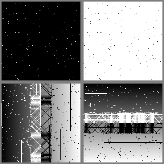
To facilitate their interpretation, the images above are obtained with a slightly
modified version of the FlowAutomaton class in order to superimpose the result
image over the source one, and to increase the contrast of the modified pixels.
Please also note that the (pseudo) random number generator was reset before
each image computation, so the initial position of the automata are the same in
each image.
From these 4 tests, one can see that the automata behave the same on the black
and the white images with 2 pixels tiny line segments. In this case, the automata
turn by 180° at each iteration alternating on the 2 pixels of the segment.
The orientation of the segment depends on the initial (random) orientation of the
automaton set by the __init__() function in the self._direction property of
the instance.
Automata also behave the same on the gradient images with respect to the gradient
orientation and, on each iteration they change their direction according to the
pixel grayscale value. We can see that the behaviour can be classified in
different kinds corresponding to similar gray levels (the two behaviours
corresponding to the black and the white are almost invisible as they only appear
on the borders of the gradient images). This is verified with the two tests below.
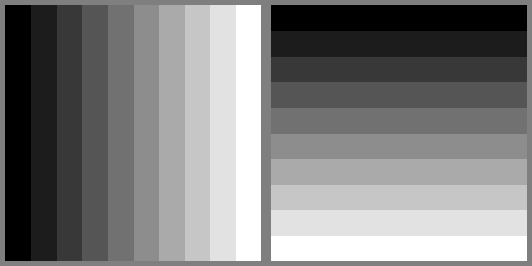
The result images show that the different behaviours are confined to the gray level strips from black to white.
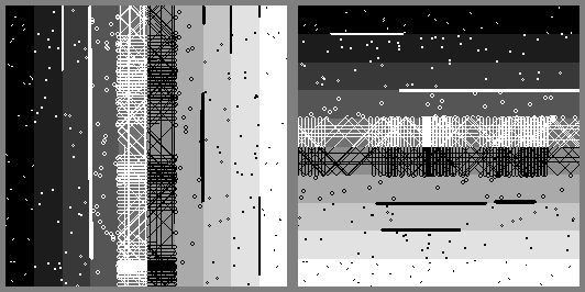
These images reveal some interesting artifacts, the automata follow the frontiers between grayscale bands.
Looking at the code
So, the direction taken by an automaton at each iteration depends on the gray level of the pixel it is laying on. The relation between the gray level and the direction is expressed with the following line of code:
self._direction = self._direction + int((gray * 8) - 4)
The direction self._direction is an integer corresponding to one of the 8 cells adjacent to the
current automata position. Direction values are numbered clockwise from 0 at the
northern position and, they are also computed modulo 8 so if direction equals 8,
it will be handled as 0, 9 as 1, and so on. This mimics the trigonometric circle
as the direction is an angle.
In the line of code above, the direction depends on the previous direction +
some change computed from the gray level variable gray, which is a float within
the [0, 1] interval. In this expression, the gray level is firstly scaled to
[0, 8] and then translated to [-4, 4].
When an automaton is on a 50% gray pixel, the gray variable equals 0.5,
int((gray * 8) - 4) equals 0, the self._direction property is left unchanged
and the automaton moves in straight line.
When an automaton is on a black pixel, the gray variable equals 0,
int((gray * 8) - 4) equals -4, the self._direction property is changed and the
automaton turns 180° before moving. The same occurs if the pixel is white as
adding 4 does the same to the direction as subtracting 4.
Other gray values change the direction by 3, 2 or 1 producing more or
less tight turns.
The behaviour appears confined to bands of similar gray level because of the integer casting. This splits the gray level interval in 9 bands:
gray |
int((gray * 8) - 4) |
|---|---|
| 0.0 | -4 |
| ]0.0, 0.125] | -3 |
| ]0.125, 0.25] | -2 |
| ]0.25, 0.375] | -1 |
| ]0.375, 0.625[ | 0 |
| [0.625, 0.75[ | 1 |
| [0.75, 0.875[ | 2 |
| [0.875, 1.0[ | 3 |
| 1.0 | 4 |
The extreme intervals are restricted to a single value while the middle one has a width twice larger than the others which have a width of one 8th.
Conclusion and perspectives
In this article we analyzed the causes of some graphic behaviour of the
FlowAutomaton class. The observed behaviour of the automata population is
driven by the data processed and, obviously, the code of the class.
Even if it’s a quite humble result, the study opens the path to other experiments.
For example, it could be interesting to add some offset (and maybe a factor) to
the pixel data in order to move the graphic effects (straight lines, curves,
dots, …) away from their corresponding grayscale bands.
It may also be possible to build some specially drawn maps to control the
trajectory of the automata as we have seen that they tend to follow the frontier
of two adjacent grayscale values.